Spectral imaging
An image can be filtered either in the frequency or in the spatial domain.
The first involves transforming the image into the frequency domain, multiplying it with the frequency filter function and re-transforming the result into the spatial domain. The filter function is shaped so as to attenuate some frequencies and enhance others. For example, a simple lowpass function is 1 for frequencies smaller than the cut-off frequency and 0 for all others.
The corresponding process in the spatial domain is to convolve the input image \(f(i,j)\) with the filter function \(h(i,j)\). Multiplication in the frequency domain is convolution in the spatial domain.
Table of Contents
1. Frequency filtering
The (discrete fourier transform) DFT is the sampled Fourier Transform and therefore does not contain all frequencies forming an image, but only a set of samples which is large enough to fully describe the spatial domain image. The number of frequencies corresponds to the number of pixels in the spatial domain image, i.e. the image in the spatial and Fourier domain are of the same size. For an NxN image, \[ F(k, l) = \sum_{a=0}^{N-1} \sum_{b=0}^{N-1} f(a,b) e^{-i2\pi(\frac{ka}{N} + \frac{lb}{N})} \], where \(f(a,b)\) is the image in the spatial domain and the exponential term is the basis function corresponding to each point \(F(k,l)\) in the Fourier space. The value of each point in \(F(k,l)\) is obtained by multiplying the spatial image with the corresponding base function and summing the result.
The basis functions are sine and cosine waves with increasing frequencies, i.e. F(0,0) represents the DC-component of the image which corresponds to the average brightness and F(N-1,N-1) represents the highest frequency.
The fourier image can be transformed back to the spatial domain using inverse fourier transform: \[ f(a,b) = \frac{1}{N^2} \sum_{k=0}^{N-1} \sum_{l=0}^{N-1} F(k,l) e^{-i2\pi(\frac{ka}{N} + \frac{lb}{N})} \]
Note that the fourier transform (FT) requires the computation of a double sum. Since the FT is separable, we can rewrite as: \[ F(k, l) = \sum_{b=0}^{N-1} P(k,b) e^{-i2\pi(\frac{lb}{N})} F(k, l) = \sum_{b=0}^{N-1} P(k,b) e^{-i2\pi(\frac{lb}{N})} \] and \[ P(k, b) = \sum_{a=0}^{N-1} f(a,b) e^{-i2\pi(\frac{ka}{N})} \]
Using this, spatial domain is first transformed into intermediate N 1-dimensional FTs. This intermediate image is then transformed into the final image again using N 1-dimensional FTs. Expressing 2-dimensional FT in terms of a series of 2N 1-dimensional transforms decreases number of required computations.
1-dimensional DFT is \(O(n^2)\), which is reduced to \(O(N lg N)\) using FFT (fast fourier transform).
The FT produces a complex number valued output image which can be displayed with two images, either with the real and imaginary part or with magnitude and phase. Often only the magnitude of the Fourier Transform is displayed, as it contains most of the information of the geometric structure of the spatial domain image.
Most implementations shift the DC-component \(F(0,0)\) such that it is the center of the frequency image. The further away from the center the pixel is, the higher is it’s corresponding frequency.
The real values of the resulting FT must also be “tone-mapped” to be visible. Usually a log-transform to re-normalize the values so that they can be seen visibly when saved/viewed.
The following shows code that will produce the FT for an image:
import cv2
import numpy as np
from matplotlib import pyplot as plt

def log_transform(img):
    c = 255.0 / np.log(1 + np.abs(np.max(img)))
    return c * np.log(1 + np.abs(img))


# load image
img = cv2.imread('bunny.jpg', 0)
# compute ft
f = np.fft.fft2(img)
# shift to move DC-component to center of fft image
fshift = np.fft.fftshift(f)
# log-transform on magnitude of FT
mag = log_transform(np.abs(fshift))

phase = log_transform(np.angle(fshift))
# show the resulting image.
plt.imshow(np.hstack([mag, phase, img]), cmap='gray')
plt.show()

Figure 1: FT of the stanford bunny image. L->R: magnitude, phase, original.
The result shows that the image contains components of all frequencies, but that their magnitude gets smaller for higher frequencies. Hence, low frequencies contain more image information than the higher ones.
The transform image also tells us that there are diagonal dominating directions in the Fourier image, one passing through the center. These originate from the regular patterns in the background of the original image.
The phase of the FT doesn’t really tell us much, but is immensely important if we ever want to recover hte original image. Below is the inverse transform on just the magnitude of the frequencies and the inverse FT of the magnitude and phase. Even though the image on the left has all the same frequencies as the original image, it is meaningless (albeit cool looking). We need both the phase and the magnitude for the inverse operation.

Figure 2: inverse FFT. Left: just magnitude. Right: magnitude and phase.
We can use these frequency images to do frequency filtering. In fact this is exactly what the gaussian filtering does. It looks like:
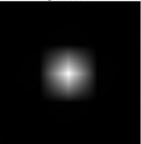
Figure 3: Gaussian in frequency space.
and kills off all higher frequencies in the input image when you multiply the gaussian with the FT of the image in frequency space.
1.1. Orienting text
A simple example: find FT of a binary english text image, threshold the frequencies and see which direction the text is flowing.

Figure 4: L->R: original text, FFT of image, FFT after thresholding frequencies.

Figure 5: L->R: original text, FFT of image, FFT after thresholding frequencies.
1.2. Image filtering
Filtering happens in the fourier domain: \[ G(k,l) = F(k,l) H(k,l) \] where \(F(k,l)\) is the input image in the Fourier domain, \(H(k,l)\) is the filter function and \(G(k,l)\) is the resulting image that can be transformed back into spatial domain using inverse FT.
Since multiplication in the Fourier domain is convolution in the spatial domain, all frequency filters can in theory be implemented as a spatial filter. However, in practice, the Fourier domain filter function can only be approximated by the filtering kernel in spatial domain.
There are 3 kinds of filters: lowpass, highpass, and bandpass.
- lowpass: a low pass filter attenuates high frequencies and leaves low frequencies unchanged. Also called a smoothing filter.
- highpass: a high pass filter does the opposite of a low pass filter. It is used to find edges in the spatial domain because edges contain many high frequencies.
- bandpass: a bandpass filter removes very high and very low frequencies and retains middle frequencies. Bandpass filtering can be used to enhance edges (suppressing low frequencies) while reducing the noise at the same time (attenuating high frequencies).
An ideal low pass filter is done by thresholding in the Fourier domain all frequencies lower than a cut-off frequency. The drawback is that such a filter is represented as a box function in the frequency domain (imagine a white box in the middle of a black image in Fourier domain). If approximating as a convolution filter in the spatial domain, we usually get ringing artifacts since that sharp edge in the frequency domain must be accounted for. Better to use the Gaussian kernel that doesn’t produce ringing artifacts.
2. LoG/Laplacian of Gaussian
Laplacian in 2-D for given image pixel intensities at \(I(x,y)\) is \[ L(x,y) = \frac{\partial^2 I}{\partial x^2} + \frac{\partial^2 I}{\partial y^2} \]
This can be discretized using finite differences to create a convolution filter that looks like the following:
|----+----+----|
|  0 | -1 |  0 |
|----+----+----|
| -1 |  4 | -1 |
|----+----+----|
|  0 | -1 |  0 |
|----+----+----|
Because these kernels are approximating a second derivative measurement on the image, they are very sensitive to noise. To counter this, the image is often Gaussian smoothed before applying the Laplacian filter. This pre-processing step reduces the high frequency noise components prior to the differentiation step.
Since convolution is associative we can convolve Gaussian kernel with Laplacian kernel to create a single kernel so we can just convolve the image once instead of once with each kernel.
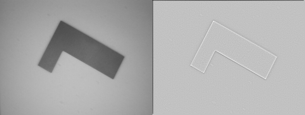
Plotting the response of the LoG kernel on a 1D image of 200 pixels:
Code that produced this image can be found here.
This clearly shows that in the vicinity of a change in intensity, LoG response will be positive on lighter side and negative on darker side. By itself, LoG filter can be used to highlight edges in an image.
3. Sampling in frequency space
We have a 1D signal, \(g(x)\) and it’s fourier transform (FT), \(G(f)\), where \(x\) is the spatial position and \(f\) is the spatial frequency. Note that \(G(f)\) are the fourier coefficients for frequencies in the entire image, we lose spatial information about where those frequencies came from in the original image.
Cleverly we can write a the sampling function like so: \[ s(x) = \sum_{n=-\inf}^{\inf}{\delta (x - n T_s)} \]
where \(\delta\) is the dirac delta function, and \(T_s\) is the sampling period, and n is the running index used with \(\delta\) to define the comb function. So if we get samples at every 10 units (\(T_s = 10\)), then δ is 1 for every 10 units of \(x\). To sample our function, we can do: \[ g_s(x) = g(x) s(x) \]
We can then take the FT of \(g_s(x)\):
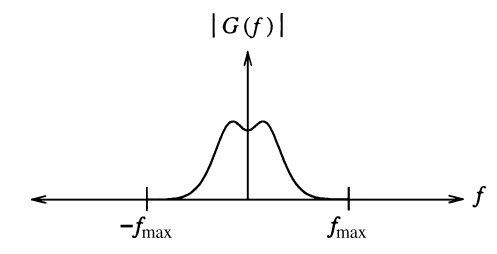
\begin{align*} G_s(f) & = G(f) * S(f) \\ & = G(f) * \left[ \sum_{n=-\inf}^{n=\inf} f_s \delta (f - f_s) \right] \\ & = f_s \sum_{n=-\inf}^{n=\inf} G(f - f_s) \end{align*}where \(f_s\) is the sampling frequency and \(*\) is convolution in frequency space. The spectrum of a signal sampled with frequency \(f_s\) (\(T_s = \frac{1}{f_s}\)) yields the original spectrum replicated in the frequency domain with period \(f_s\). This property has important consequences. It yields a spectrum \(G_s(f)\) that is periodic in frequency with period \(f_s\).
A small sampling period is equivalent to a high sampling frequency, yielding spectra replicated far apart from each other. In the limit, as \(T_s \rightarrow 0, f_s \rightarrow \inf\), only a single spectrum appears, consistent with the continuous case resembling the original signal.
3.1. Reconstruction
To reconstruct the sampled signal, we can break up our \(G_s(f)\) as \[ G_s(f) = G(f) + G_{high}(f) \] where \(G(f)\) is the original signal we want to reconstruct and the \(G_{high}(f)\) is the replicated versions of \(G(f)\).
For exact reconstruction we need the following conditions to hold:
- \(G(f)\) must be band limited, not have a spectra of infinite extent.
- Sampling frequency \(f_s\) must meet the nyquist limit. Intuitively this states that the minimum distance between spectra copies in \(G_s(f)\) must be at least \(f_{max}\) apart, setting the nyquist limit to \(f_s > 2 f_{max}\). \(f_{max}\) is the maximum frequency extent of \(G(f)\). If we don’t meet hte nyquist limit, then we are undersampling, and the spectra copies overlap each other, causing aliasing.
The ideal reconstruction strategy is to remove \(G_{high}(f)\) completely, which can be done with an ideal low pass filter \(H(f)\) such that: \[H(f) = \left\{ \begin{array}{l l} 1, & \quad |f| < f_{max} \\ 0, & \quad |f| \geq f_{max}\\ \end{array} \right. \]
The ideal low pass filter will supress all frequencies above \(f_{max}\) effectively disregarding \(G_{high}(f)\) and only leaving the original signal \(G(f)\). \(G(f) = H(f) \cdot G_s(f)\).
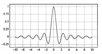
In the spatial domain the ideal low pass filter is the sinc function. IFT of \(H(f)\) is \[ sinc(x) = \frac{\sin(\pi x)}{\pi x} \] The reader should note the reciprocal relationship between the height and width of the ideal low-pass filter in the spatial and frequency domains. Let A denote the amplitude of the sinc function, and let its zero crossings be positioned at integer multiples of 1/2W. The spectrum of this sinc function is a rectangular pulse of height A/2W and width 2W, with frequencies ranging from −W to W. In our example above, A = 1 and W = \(f_{max}\) = 0.5 cycles/pixel. This value for W is derived from the fact that digital images must not have more than one half cycle per pixel in order to conform to the Nyquist rate.
We can reconstruct the signal in spatial domain using convolution with the sinc function \[ g(x) = sinc(x) * g_s(x) \]
Ideal low-pass and the sinc function are not practical as they require infinite number of neighboring samples in the spatial domain. One can try to truncate the sinc function, but this leads to ringing artifacts. This is known as the Gibbs phenomenon, which are overshoots and undershoots caused by reconstruction of a signal with truncated frequency terms. Truncation in the spatial/frequency domain leads to ringing in the other domain.
The accuracy of a reconstruction filter can be evaluated by analyzing its frequency-domain characteristics. Of particular importance is the filter response in the passband and stopband. In this problem, the passband consists of all frequencies below \(f_{max}\). The stopband contains all higher frequencies arising from the sampling process.
Imperfect filtering on the passband will result in some sort of smoothing/blurring or sharpening on the image as we have not replicated the original signal’s frequencies properly.
If the stopband is allowed to persist, then this constributes to aliasing – additional frequencies folding over into the passband range.
One can think of interpolation as simply convolution in the spatial domain. The kernel is centered at x, the location of the point to be interpolated. The value of that point is equal to the sum of the values of the discrete input scaled by the corresponding values of the reconstruction kernel. This follows directly from the definition of convolution.
The Lancos filter is modeled after the sinc function, but attempts to reduce the ringing artifacts resulting from naive truncation.
3.2. Aliasing
There is a misconception that jagged (staircased) edges a symptom of aliasing. This is only partially true. Technically, jagged edges arise from high frequencies introduced by inadequate reconstruction. Since these high frequencies are not corrupting the low-frequency components, no aliasing is actually taking place. Remember that aliasing is the overlap of frequencies created from undersampling the signal, See Figure 10.
This confusion exists because the suggested solution is to increase the sampling rate, which is also a solution to reduce aliasing. The benefit of increasing the sampling rate is that the replicated spectra are now spaced farther apart from each other which in turn relaxes the accuracy constraints for reconstruction filters to perform ideally in the stopband, where they must suppress all components beyond some specified cutoff frequency. Increasing the sampling rate results in the same nonideal filters producing less objectionable output.
It is important to note that a signal may be densely sampled (far above the Nyquist rate) and continue to appear jagged if a zero-order reconstruction filter is used. Box filters used for pixel replication in realtime hardware zooms are a common example of poor reconstruction filters. In this case, the signal is clearly not aliased but rather poorly reconstructed.
The distinction between reconstruction and aliasing artifacts becomes clear when we notice that the appearance of jagged edges is improved by blurring. This is a defocusing operation that attenuates the high frequencies admitted through nonideal reconstruction. On the other hand, once a signal is truly undersampled, no postprocessing will improve its condition. After all, applying an ideal low-pass (reconstruction) filter to a spectrum whose components are already overlapping will only blur the result, not rectify it.
3.3. Antialiasing
To combat aliasing, a common approach is to prefilter the signal such that it bandlimits the signal to values less than \(f_{max}\), thereby eliminating offending high frequencies.
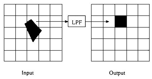
Area filtering for example: Rather than sampling a point, instead apply a low-pass filter (LPF) upon the projected area in order to properly reflect the information content being mapped onto the output pixel. The low-pass filter comprises the prefiltering stage. It serves to defeat aliasing by bandlimiting the input image prior to resampling it onto the output grid.
The process of using more than one regularly spaced sample per pixel is known as supersampling. Each output pixel value is evaluated by computing a weighted average of the samples taken from their respective preimages. For example, if the supersampling grid is three times denser than the output grid (i.e., there are nine grid points per pixel area), each output pixel will be an average of the nine samples taken from its projection in the input image. If, say, three samples hit a green object and the remaining six samples hit a blue object, the composite color in the output pixel will be one-third green and two-thirds blue, assuming a box filter is used. Supersampling reduces aliasing by bandlimiting the input signal. The samples then enter the prefiltering stage, consisting of a low-pass filter. This permits the input to be resampled onto the (relatively) low-resolution output grid without any offending high frequencies introducing aliasing artifacts.
4. DCT
Another sinusoidal transform (i.e. transform with sinusoidal base functions) related to the DFT is the Discrete Cosine Transform (DCT).
The main advantages of the DCT are that it yields a real valued output image and that it is a fast transform. A major use of the DCT is in image compression — i.e. trying to reduce the amount of data needed to store an image. After performing a DCT it is possible to throw away the coefficients that encode high frequency components that the human eye is not very sensitive to. Thus the amount of data can be reduced, without seriously affecting the way an image looks to the human eye.
5. Nonlinear filters
Suppose that an image processing operator F acting on two input images A and B produces output images C and D respectively. If the operator F is linear, then
\[ F(a * A + b * B) = a*C + b*D \] where \(a\) and \(b\) are constants. This property doesn’t hold for nonlinear filters. The median filter for example is nonlinear, since \[ median(A(x) + B(x)) \neq median(A(x)) + median(B(x)) \]

